What Is an Electronic Board and How Does It Work?

An electronic board is a compact platform that connects components, controls signals, and manages electrical power. It may refer to a printed circuit board, a control board, or a specialized circuit assembly. Each type serves a different purpose. However, all rely on carefully designed electrical paths.

Copper traces carry current between components such as resistors, capacitors, processors, sensors, and connectors. When power enters the board, voltage reaches the required circuits through these paths. A processor may then interpret sensor data and send commands to motors, displays, or communication modules. The board’s behavior depends on component values, wiring layout, firmware, and operating conditions.

Small details matter.

From a repair and design perspective, heat, moisture, vibration, and poor connections can change performance. A loose connector may cause intermittent faults. A damaged trace can stop an entire system. Testing with a multimeter, oscilloscope, or inspection camera often reveals problems that are invisible at first glance. Yet diagnosis is not always straightforward. Similar symptoms can come from different failures, and one mistaken assumption can lead to unnecessary component replacement.

This article explains what an electronic board is and how it works in real applications. It explores board structure, power distribution, signal movement, component roles, and common failure points. The discussion uses practical engineering principles while recognizing that board designs vary widely. A simple household controller and an industrial automation board may follow the same fundamentals, but their safety requirements differ. Understanding those fundamentals makes technical documentation easier to read and troubleshooting more systematic.
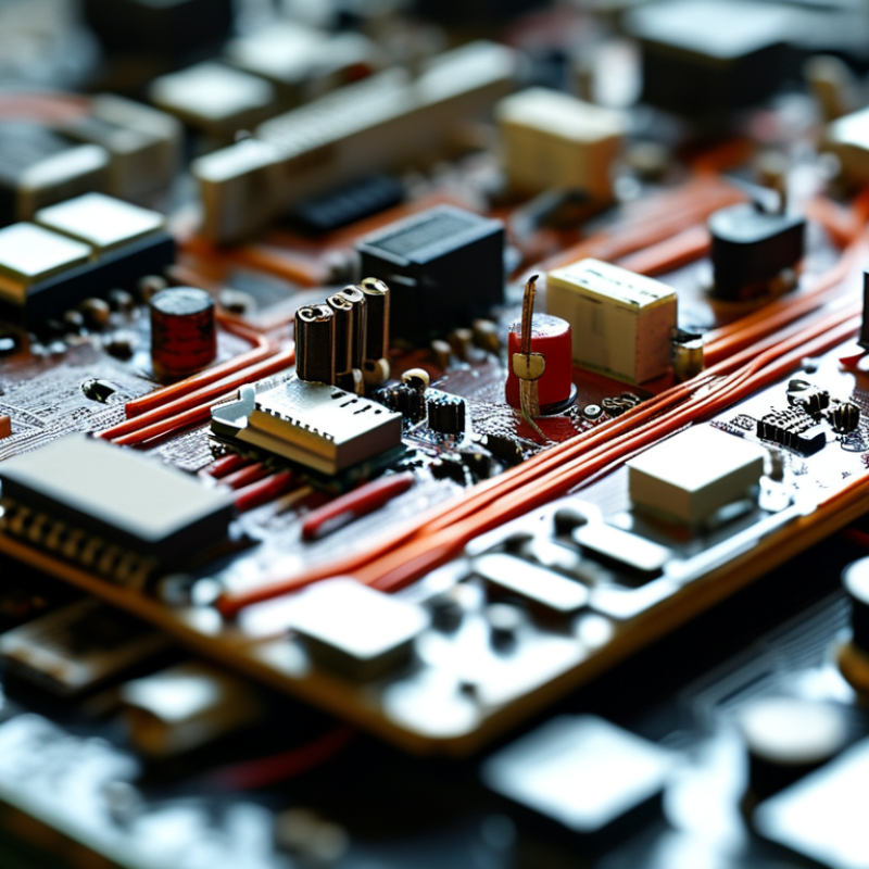
What Is an Electronic Board and How Does It Work?

Electronic Board Types and the IPC Standards That Define Their Roles

An electronic board is a structured platform that connects components through conductive paths. It controls power, signals, and data inside equipment. Common types include rigid, flexible, rigid-flex, high-density interconnect (HDI), and metal-core boards. Each type fits a different physical and thermal challenge. Flexible circuits bend around hinges. Rigid boards support stable, high-volume assembly. HDI boards use microvias and fine lines for compact products.

IPC standards help define these roles with measurable requirements. IPC-2221 provides general design guidance, while IPC-6012 covers rigid board qualification. IPC-6013 addresses flexible circuits, and IPC-6016 focuses on HDI structures. IPC-A-600 describes board acceptability, including conductor edges, plating, and laminate conditions. Assembly teams often use IPC-A-610 to judge soldered results. These documents do not merely decorate a specification. They guide inspection, testing, and supplier communication.

Market data shows why this discipline matters. A 2024 Mordor Intelligence report estimated the global PCB market at about 76.9 billion U.S. dollars, with projected growth toward 109.5 billion by 2029. IPC’s North American PCB Statistical Program also tracks monthly sales and order trends, showing how quickly demand can shift. Numbers vary by research method. That is worth remembering. A board may pass visual inspection yet fail under vibration, moisture, or repeated bending. Real engineering experience still requires testing the finished design, not trusting the drawing alone.
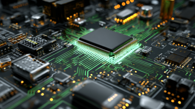

What Is an Electronic Board and How Does It Work?

Electronic boards use conductive copper paths, insulating materials, and mounted components to route power and signals. Their construction and performance are described by IPC design and qualification standards.

Nominal copper thickness is approximately 35 micrometres per ounce per square foot. Finished board thickness may vary because of plating, etching, manufacturing tolerances, and the selected material system.

Rigid Boards

Solid substrates support components and maintain a fixed shape. IPC-6012 defines qualification and performance requirements for many rigid printed boards.

Flexible Boards

Flexible circuits use bendable dielectric materials for compact or moving assemblies. IPC-6013 addresses qualification and performance requirements for flexible printed boards.

IPC Product Classes

Class 1 covers general products, Class 2 covers dedicated-service products, and Class 3 covers high-reliability products where continued performance is critical.

How it works: Copper traces connect components into electrical circuits. Dielectric layers isolate conductors, vias connect different layers, and the chosen IPC class establishes the inspection and performance expectations for the intended application.

Layer Stackup: How 35 μm Copper Traces Carry Electrical Signals

An electronic board connects components through patterned copper layers. These paths carry power, timing signals, and data between devices. In a typical board, 35 μm copper is close to one ounce per square foot. It sounds thin. Yet it can carry useful current when trace width, temperature, and copper distribution are properly controlled.

Layer stackup decides how signals behave. A four-layer board may place signal layers beside a continuous ground plane. This short return path reduces loop area and unwanted radiation. The dielectric thickness between layers also affects impedance. A wider trace usually lowers impedance, while greater spacing can reduce crosstalk. Engineers calculate these values before fabrication, then verify critical dimensions on test coupons.

Heat changes the picture. Narrow 35 μm traces can warm quickly near connectors, vias, or power components. Wider copper pours spread heat and reduce resistance. Vias must also support the expected current; one small via may become a bottleneck. In practical inspections, solder mask thickness, etching variation, and uneven plating deserve attention. The drawing may be correct, but the finished board can still differ slightly. That gap needs measurement, not assumption.

What Is an Electronic Board and How Does It Work? - Layer Stackup: How 35 µm Copper Traces Carry Electrical Signals
Data Category Parameter Representative Value Engineering Meaning
Copper Layer Nominal copper thickness 35 µm (0.035 mm) A common finished copper thickness for a printed circuit board layer. It is approximately equivalent to 1 oz/ft² of copper, whose nominal thickness is about 34.8 µm.
Copper Layer Approximate thickness in mils 1.38 mil This is the same physical thickness expressed in imperial units.
Material Property Copper resistivity at 20 °C Approximately 1.68 × 10⁻⁸ Ω·m Lower resistivity allows copper traces to conduct electrical current with relatively low power loss.
Trace Resistance Sheet resistance of 35 µm copper Approximately 0.48 mΩ/square Calculated from resistivity divided by copper thickness. One electrical square has the same resistance regardless of its absolute size.
Trace Resistance 1.00 mm wide × 100 mm long trace Approximately 48 mΩ The trace contains 100 squares because its length is 100 times its width. The value is a room-temperature DC estimate before temperature rise and surface effects.
Trace Resistance 0.20 mm wide × 100 mm long trace Approximately 240 mΩ The narrower trace contains 500 squares, so it has about five times the resistance of a 1.00 mm wide trace with the same length and copper thickness.
Power Loss Voltage drop at 1 A through the 1.00 mm trace Approximately 48 mV Calculated using V = I × R. The value increases if the copper becomes hotter because copper resistance rises with temperature.
Power Loss Heat generated at 1 A through the 1.00 mm trace Approximately 48 mW Calculated using P = I2R. Actual temperature rise depends on trace width, surrounding copper, board thickness, airflow, and allowed temperature rise.
Illustrative Stackup Layer 1 35 µm copper Outer signal layer. Components and high-speed traces may be placed on this layer.
Illustrative Stackup Dielectric between Layers 1 and 2 0.20 mm nominal The dielectric separates the signal layer from its closest reference plane. Its thickness strongly affects controlled impedance.
Illustrative Stackup Layer 2 35 µm copper ground plane A continuous reference plane provides a low-inductance return path and helps reduce electromagnetic emissions when signal routing remains above the plane.
Illustrative Stackup Core dielectric between Layers 2 and 3 0.80 mm nominal The core provides mechanical support and electrical insulation between the internal copper layers.
Illustrative Stackup Layer 3 35 µm copper power plane A power plane distributes supply voltage. It is normally paired with a nearby ground plane to reduce loop inductance and high-frequency noise.
Illustrative Stackup Dielectric between Layers 3 and 4 0.20 mm nominal This insulating layer separates the internal power plane from the bottom signal layer.
Illustrative Stackup Layer 4 35 µm copper Bottom signal layer. It can carry slower signals, routing, or additional connections depending on the circuit layout.
Illustrative Stackup Approximate finished board thickness 1.34 mm, excluding solder mask Calculated from four 35 µm copper layers plus 1.20 mm of stated dielectric material. Real manufacturing thickness varies with resin content, copper plating, and process tolerances.
Signal Behavior Primary factors affecting trace impedance Trace width, copper thickness, dielectric height, dielectric constant, and solder mask A 35 µm copper thickness alone does not define impedance. The complete stackup and trace geometry must be specified for controlled-impedance routing.
Signal Return Preferred high-frequency return path The nearest continuous reference plane High-frequency return current tends to follow the path of lowest inductance directly beneath the signal trace. Gaps or slots in the reference plane can force a longer and noisier return path.
Current Capacity Maximum allowable current Not determined by copper thickness alone Safe current depends on trace width, external or internal location, permissible temperature rise, ambient conditions, nearby copper, and the applicable design rules.
Electrical Function How the copper trace carries a signal Voltage and current travel through a defined conductor and return path The copper trace provides a low-resistance path for charge movement. The surrounding dielectric controls electric-field distribution, while reference planes provide the return path and help control signal integrity.
Values marked as representative or nominal are engineering examples rather than universal manufacturing requirements. Resistance calculations use copper resistivity at 20 °C and exclude connector, via, plating, surface-finish, and temperature effects.

From Schematic to PCB: IPC-2221 Rules for Routing and Spacing

An electronic board turns electrical intent into a physical circuit. The schematic defines connections, while the PCB controls distance, heat, noise, and manufacturability. IPC-2221 provides a practical framework for moving between these stages. It helps engineers consider conductor width, insulation spacing, dielectric materials, and voltage stress. However, its values are not a substitute for engineering judgment. Voltage, altitude, pollution level, coating, and operating environment can change the required clearance.

A reliable layout begins by assigning net classes before routing. High-voltage nets need wider clearance from nearby conductors, mounting holes, and exposed copper. Creepage follows the board surface, while clearance crosses the air gap. They are different measurements. Sensitive signal traces should stay away from fast switching nodes and use a continuous return path. Differential pairs need controlled spacing and consistent geometry, but the exact dimensions depend on the stackup and impedance target. IPC-2221 also encourages practical attention to vias, copper widths, and thermal reliefs. Small details matter. During a design review, a neat route can still hide a weak return path or an accidental copper island. I sometimes leave more space than the minimum because production variation, dust, and inspection errors are real. Minimum spacing may pass the drawing and fail the factory. A final review should compare the layout with the current standard, manufacturer capability, safety requirements, and actual test results.

Component Assembly: SMT Placement and IPC-A-610 Acceptance Criteria

What Is an Electronic Board and How Does It Work?

Component Assembly: SMT Placement and IPC-A-610 Acceptance Criteria

An electronic board connects components through copper traces, allowing signals and power to move between circuits. In SMT assembly, solder paste is printed onto small pads before automated placement begins. A pick-and-place machine positions resistors, capacitors, and integrated circuits with measured precision. Reflow heating then melts the paste and forms permanent solder joints.

I have inspected assemblies where one shifted component stopped an entire board from working. Placement accuracy matters, but paste volume matters too. Excess paste can create solder bridges between fine-pitch pins. Too little paste may produce weak joints or incomplete wetting. Operators check alignment, polarity marks, lifted leads, and tombstoning after reflow. Optical inspection helps, although it cannot reveal every hidden connection.

IPC-A-610 provides visual acceptance criteria for electronic assemblies. Its requirements differ by product class, inspection point, and component type. Inspectors evaluate solder fillets, lead coverage, terminal contact, cleanliness, and visible defects. Class 3 usually demands the highest assurance for critical equipment. X-ray inspection may support checks beneath bottom-terminated components, but it should not replace process control. A board can pass visual inspection and still deserve deeper review. That uncomfortable gap is why records, calibrated tools, and trained judgment remain essential. Mistakes happen. The process must expose them early.

Power-Up to Data Transfer: Why FR-4 Signals Travel About 15 cm/ns

An electronic board is a layered platform that powers components and directs electrical signals. Copper paths connect processors, memory, sensors, and connectors. When power rises, tiny voltage changes begin moving through those paths.

On FR-4, a signal travels about 15 centimeters per nanosecond. This figure describes electromagnetic propagation, not electrons racing from one component to another. The speed is lower than light in air because the circuit material stores electric energy. Its effective dielectric constant, trace geometry, and nearby reference plane all affect the result.

A 30-centimeter trace may therefore add roughly two nanoseconds of travel time. That sounds negligible. It is not always negligible. Fast digital edges can contain frequency components far above their stated clock rate. A short trace may then behave like a transmission line, producing reflections when impedance changes suddenly. Vias, connectors, narrow necks, and poorly placed returns can disturb the waveform.

In practical board analysis, I check the complete signal path rather than trusting a single speed estimate. The 15 cm/ns value is useful, but imperfect. FR-4 is not electrically uniform across every stack-up. Resin content, glass weave, trace width, and layer spacing can shift propagation delay. A measurement may also disagree with a simplified calculation.

Clean data transfer depends on controlled impedance, continuous return paths, suitable termination, and careful timing margins. Power integrity matters too. A noisy supply can distort the same edge that the data receiver is trying to interpret. Small details become visible quickly.